Assignments

Each assignment applies one of the models that we studied in class to a real world question. The answer should be a document about 4 pages in length.

A good answer does not just apply the model mechanically to the problem. It also thinks about aspects that the model misses and modifies the answer accordingly.

Be sure to really explain your answer. In your graphs, explain which curves shift, by how much, and why. Explain the economic process that leads to the changes depicted in the graph.

How to submit

Please submit your submission via Gradescope any time prior to midnight of the due date.

Hand-written documents are fine, but make sure I can read them.

If you submit an image, please use scanning software. Do not submit photos (those are hard to read).

Example

Suppose that the interest elasticity of investment rises. Does this make monetary and fiscal policy more or less effective?

Since we are working in an IS/LM framework, we start with the model equations:

1. IS: \(Y=\bar{Z} + (b_1 + c_1)Y - b_2 i\)
2. LM: \(M/P = Y \times L(i)\)

We are considering how a higher \(b_2\) changes the effects of a given change in \(G\) or \(M\).

How does a higher \(b_2\) change the graph?

Let's write IS as \(i = \frac{\bar{Z} - (1 - b_1 - c_1) Y}{b_2}\). A higher \(b_2\) makes the IS curve flatter. The intuition is as follows. Starting from a point on IS, suppose we raise \(Y\). That moves us to the right of the IS curve where we have excess supply of goods (a unit increase in \(Y\) only leads to an increase in demand of \([1-b_1-c_1]\)). A lower \(i\) is required for goods market clearing. If \(b_2\) is high, a small drop in \(i\) leads to a large increase in \(I\) and is sufficient to restore market clearing. Therefore, IS is flat.

The value of \(b_2\) also affects the intercept of IS, but we do not care about that right now.

Fiscal shock

Increasing government spending by \(\Delta G\) shifts IS to the right by \(\frac{\Delta G}{1 - b_1 - c_1}\), which is independent of \(b_2\). Note: if we considered the vertical shift, \(\Delta G / b_2\), it would depend on \(b_2\) which makes life harder.

We may now compare the effects of a given change in \(G\) for high and low elasticities \(b_2\). To do so, we draw an IS/LM diagram with one LM curve and two IS curves that intersect LM in the same point (for easy visualization).

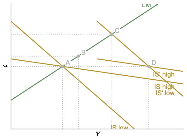
The economy starts at point A in both cases. The IS curves shift right by a given amount, so they intersect at point D. The new equilibria are given by B (high elasticity) and C (low elasticity). In the high elasticity (flat IS) case, output rises less.

Now we turn to the intuition. Starting at A, higher \(G\) raises demand and therefore output to point D (in both cases). At D we have excess demand for money. Households sell bonds, which drives up the interest rate. Higher interest rates crowd out investment and output starts to fall.

If investment responds strongly to interest rates, this crowding out effect is strong. A given increase in \(i\) causes a large decline in demand and therefore \(Y\). This is why the equilibrium increase in \(Y\) is small when investment is interest sensitive.

So the basic intuition is really very simple (but hard to see clearly without the model): A shock to aggregate demand causes interest rates to rise. Crowding out dampens the increase in output. If demand is interest sensitive, crowding out is strong.

Monetary shock

A similar write-up would go here...

---